Visual Tracking papers

Visual Tracking Review

Author: Ferhat Can ATAMAN
Created In 06/04/2020
Last Modified: 07/04/2020

Aim of this review is to investigate some of the core visual tracking papers that give solutions to basic problems in area. Before going on deep learning methods, these review can give good intuition about the field.

---

Core papers

• Average of Synthetic Exact Filters (ASEF) CVPR09
• Visual Object Tracking using Adaptive Correlation Filters (MOSSE) CVPR10
• Target Aware Deep Tracking (TADT) CVPR19

1. ASEF (CVPR09)

It tries to solve robustness problem. That is changing in the appearance should not effect results of the localization. There should be training set to learn custom correlation filter.

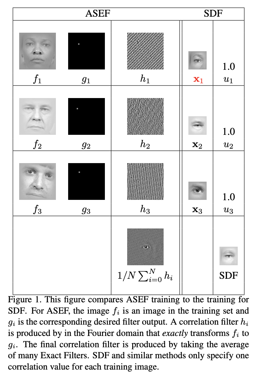
Fig.1: ASEF algorithm explanation

• Correlation between the image and filter should give single peak (impulse) response in correlation plane. This peak is the center of our object. (In this paper, the object is the eye localization)
  • However, in real life, relative peak strength of responses to changing targets can be unpredictable. Instead of using ideal impulse response in the desired output, Gaussian shape response is used.
  $$g_i(x, y) = e^{\frac{(x - x_i)^2 + (y - y_i)^2}{\sigma^2}}$$ $$(x, y): center\, of\, eye\, in\, training\, images$$
  • The closer points to the center of eye have higher coefficients and these coefficients’ decay rate is decided with $\sigma$.

• After generating desired outputs for dataset, (that is $g_i(x,y)$ for $i^{th}$ training example) exact correlation filters are found.

  $$g(x, y) = (f \otimes h)(x, y)$$ $$f(x, y): training\, example, \quad h(x, y): filter$$
  • Convolution in spatial domain is equal to element-wise multiplication in Fourier Domain.
  $$G(w, v) = F(w, v)H^*(w,v) \rightarrow H^*(w, v) = \frac{G(w, v}{F(w, v)}$$

  • Filters are found in Fourier domain. Each filter gives exact result on each corresponding training image. It can be considered as weak classifiers. This method called as bagging. If weak classifiers are unbiased, their summation converges upon a classifier with zero variance error.

  • Exact filters can be averaged in both Domain. If exact filters are in spatial domain, they can be cropped before averaging which allows ASEF filters can be constructed from different size training images.

  $H^*_\mu(w, v) = \frac{1}{N}\sum_{i=1}^N H^*_i(w, v) **$ $h_\mu(x, y) = \frac{1}{N} \sum_{i=1}^N h_\mu(x, y) **$

  • A single robust filter is obtained to determine position of the target at arbitrary image.

• To find ASEF filter, RST(Rotation, Scale, Translation) is applied to augment dataset and it makes filters more reliable.

  • All images are normalized to remove some effects.

    • $log(log(v + 1))$ normalization applied to the pixel values to reduce effects of shadows and intense lighting.
    • Normalize images to give 0.0 mean and 1.0 squared sum to obtain consistent intensity values.
    • Cosine window (?) is applied to reduce frequency effects of the edge of the images when transformed by FFT(fast Fourier transform).

2. MOSSE (CVPR10)

It tries to solve visual tracking problem with using correlation filters that is similar to ASEF. In this approach, correlation filter is updated online according to current target appearance. The target window is selected in first frame of the video, then MOSSE initializes tracking. First, the initial MOSSE filter is constructed with target window and its’ N (hyperparameter) affine permutations like Rotation, Scale and Translation (RST). After that, in each frame, MOSSE filter updating with moving average that is new filter has smaller effect than early calculations.

Two main contribution exist:

• Smaller number of training dataset can be used.
• Filter can be updated online that increases adaptation ability of the approach when the appearance of the target changes in time.

ASEF needs too much training sample to obtain reliable correlation filter $H(w, v)$. (When we have small number of train data, element-wise division in frequency domain can be unstable. The reason behind this the training image contains very little energy that is $F_i \odot F_i^$ closes to zero.) It becomes too slow for tracking purpose.

$$H_i^* = \frac{G_i}{F_i} = \frac{G_i \odot F_i^* }{F_i\odot F_i^* } \quad ...ASEF$$

• MOSSE FILTER: The approach of obtaining correlation filter in MOSSE is different from ASEF. For whole training sample, minimum squared error solution is tried to find.

  • Firstly, optimization problem is defined as below:
  $$\min_{H^* } \sum_{i}\left| F_i \odot H^* - G_i \right| ^2$$
  • Then to find optimal $H^{* }$, take derivative of above formula and equalize to zero.
  $$0 = \frac{\partial}{\partial H_{wv}^{* }} \sum_{i}\left| F_{iwv} \odot H^{* }_{wv} - G_{iwv} \right|^2$$ $$0 = \frac{\partial}{\partial H_{wv}^{* }} \sum_i (F_{iwv} \odot H^{* }_{wv} - G_{iwv}) (F_{iwv} \odot H^{* }_{wv} - G_{iwv})^{* }$$ $$0 = \frac{\partial}{\partial H_{wv}^{* }} \sum_i F_{iwv}F_{iwv}^{* }H_{wv}H_{wv}^{* } - F_{iwv}G_{iwv}^{* }H_{wv}^{* } - F_{iwv}^{* }G_{iwv}H_{wv} + G_{iwv}G_{iwv}^{* }$$ $$H_{wv} = \frac{\sum_i F_{iwv}G_{iwv}^{* }}{\sum_i F_{iwv}F_{iwv}^{* }}$$
  • Then, rewrite above result in array notation:
  $$H_{i} = \frac{\sum_i F_{i} \odot G_{i}^{* }}{\sum_i F_{i} \odot F_{i}^{* }}$$
  • We need to find $H^{* }$ so;
  $$H_{i}^{* } = \frac{\sum_i G_{i} \odot F_{i}^{* }}{\sum_i F_{i} \odot F_{i}^{* }} \quad ...MOSSE$$
  • There are some interesting results in this derivation. The numerator is the correlation between the input and desired output and the denominator is the energy spectrum of the input.

• MOSSE is more stable than ASEF when there is smaller training set. Because, when there is an sample with low energy level, it makes denominator of the ASEF formula to zero. When same case occurs in MOSSE, because of sum of samples is calculated, the denominator rarely becomes smaller number that causes unstability.

• ONLINE UPDATES: Moving average algorithm is used to update filter.

  • For ASEF filters:
  $$H_i^{* } = \eta\frac{G_i \odot F_i}{F_i \odot F_i^{* }} + (1 - \eta)H_{i-1}^{* }$$
  • For MOSSE filter:
  $$H_i^{* } = \frac{A_i}{B_i}$$

  $A_i = \eta (G_i \odot F_i) + (1 - \eta)A_{i-1}$ $B_i = \eta (F_i \odot F_i^{* }) + (1 - \eta)B_{i-1}$

  • 0.125 is recommended for $\eta$(learning rate).

• FAILURE DETECTION & PSR: Peak to sidelobe ratio (PSR) is calculated to measure peak strength of correlation result. Maximum peak value $g_{max}$, sidelobe mean $\mu_{sl}$ and standart deviation $\sigma_{sl}$ is calculated from correlation output $g$. Sidelobe is the whole correlation output excluding the peak and its’ 11x11 neighborhood pixels.

$$PSR = \frac{g_{max} - \mu_{sl}}{\sigma_{sl}}$$

• When PSR is higher than 20, it shows the peak is strong. When PSR drops to 7, it means target is occluded or tracking has failed.

3. TADT (CVPR19)

The main purpose of this approach is following. Pre-trained CNN that is trained for object classification task can be used to extract features of an object. However, the classification network have tendency to separate inter-class differences. In tracking scenarios, tracking objects can be in same class. That is there could be 2 person crossing each other. In single target tracking, the intra-class separation is also important. Thus, from pre-trained network, features that mostly activate our desired object can be found. If we found these features, to track object, only these features can be used to localize object location on the next frame. For feature comparison, Siamese matching network is used.

Basically, the important features should be selected using following equation: $\chi^{‘} = \varphi(\chi;\Delta)$. $\chi$ is input features and $\varphi(.)$ function selects important features according to the channel importance, $\Delta$.

$$\Delta_i = G_{AP}(\frac{\partial L}{\partial z_i})$$

where $G_{AP}(.)$ global average pooling function, $L$ is the loss function to select features and $z_i$ is the output feature of $i^{th}$ filter.

There are 2 loss function to select important features. Target active features via regression loss and Scale sensitive features via ranking loss.

For the given object, firstly, pre-trained features are calculated. Then, losses are calculated and gradients are found to select features using above equations.

• Regression Loss($L_{reg}$): In feature maps, object regions are activated and background regions are surpassed. A simple regression network is designed to activate object regions only. To do that, we should fit the the regression network to give desired output. Inputs are feature channels and desired output can be considered as a 2D Gaussian with a peak at object center and have a sigma,$\sigma$, to determine spread of the Gaussian function. This simple regression network is trained using ridge regression loss in blow equation where $Y(i,j)$ is the desired output, $X_{i,j}$ a feature channel and $W$ is the weights that is learned.

$$Ridge\, Regression\, Loss \rightarrow L_{reg} = \| Y(i, j) - W * X_{i, j}\|^2 + \lambda\|W\|^2$$

• With gradient of ridge regression loss wrt. input channel becomes input to $G_{AP}(.)$ function.

$$\frac{\partial L_{reg}}{\partial x_{in}} = \sum_{i, j} 2(Y(i, j) - W * X_o(i, j)) \times W$$

• Ranking Loss($L_{rank}$): It tries to find scale sensitive features. To do that, a network is defined. $f(x;w)$ predict scales. Training samples are collected from features from different scales. Then, pairwise comparison is done to calculate ranking loss.

$$Rankin\, Loss\, \rightarrow L_{rank} = log(1 + \sum_{(x_i, x_j) \in \Omega} exp(f(x_i) - f(x_j)))$$ $$\frac{\partial L_{rank}}{\partial x_{in}} = \frac{\partial L_{rank}}{\partial f(x_{in})} \times W$$

WARNING: This part can be more clear. In paper, it is not explained very well. The inspired paper should be read.

Above loss calculating networks to select important feature channels are trained with first frame of the tracking sequence. Thus, in initializing phase, target aware features from pre-trained network are decided and after these process, until the end of the tracking, same feature channels are used.

• For Siamese matching network, current target and search space to localize target in the current frame are given. Target search space is 3 times larger than the target dimensions. Initial target, $x_1$ and search region in current frame, $z_t$, predicted target position in frame t is calculated as below:

$$I = \arg\max_{p}\chi^{'}(x_1) * \chi^{'}(z_t)$$

where ${* }$ denotes convolution operation.

Overall network architecture in the paper is shown in Fig.2. Dashed part is calculated only in initialization part.

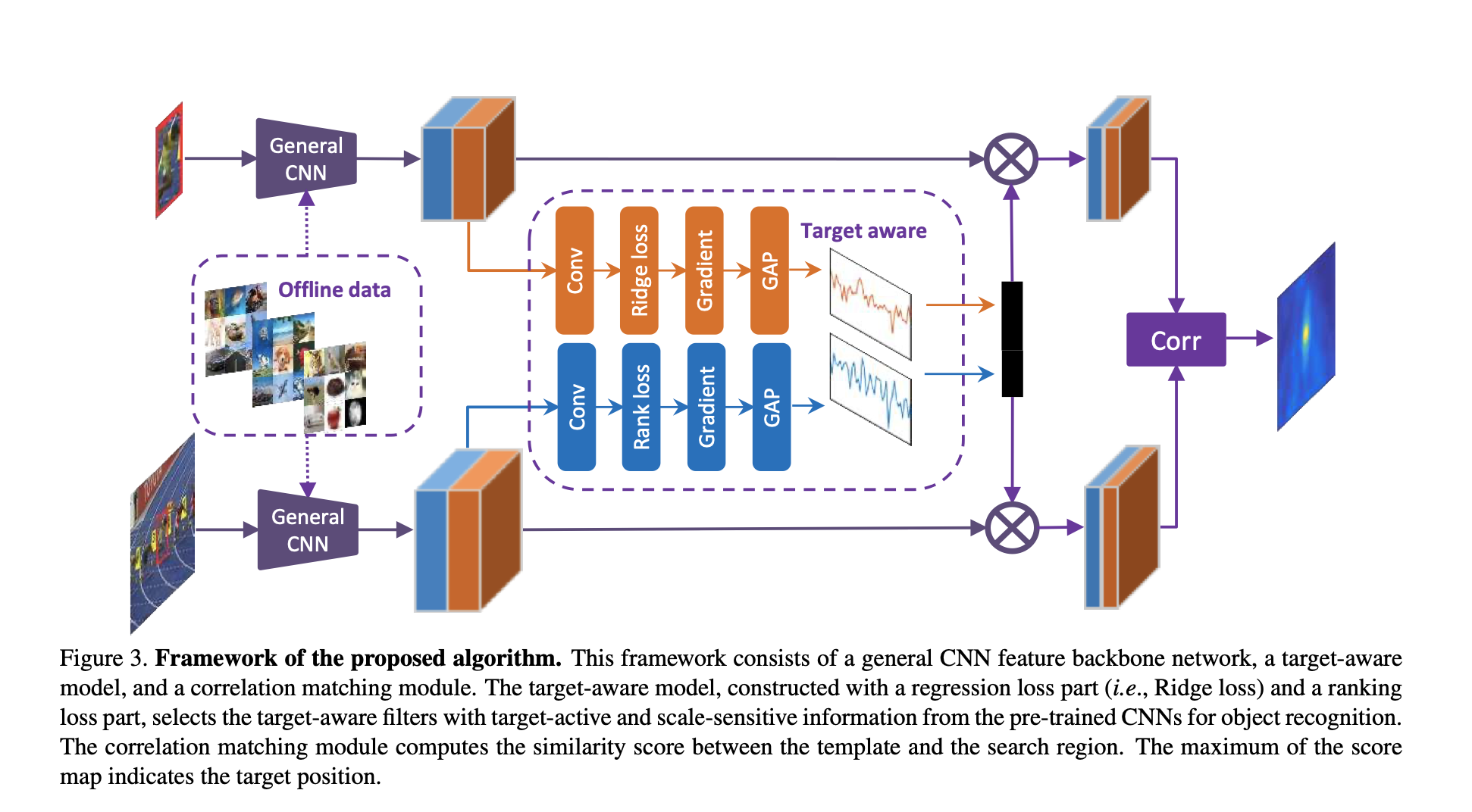
Fig.2: TADT algorithm explanation

To conclude, this method does not obtain best accuracy on dataset but it is very fast compared to other methods.